BEM For Helmholtz Sound-Soft Scattering Problem

During the course of Advanced Numerical Methods for PDE we study the Boundary Elements Method (BEM) for the solution of the Sound Soft Scattering Problem, this post is a remake of the report I presented as part of the exam.

We fix the notation that we will use from now on in this report, let $\Omega_{-}\subset \mathbb{R}^2$ be a bounded Liptschitz domain and $\Omega_{+}$ the complement of its closure in $\mathbb{R}^2$ . We require $\Omega_{-}$ to be simply connected.
Let us recall the Helmholtz PDE, that is gonna be the focus of our report:

$\Delta u + k^2 u=0$

Definition – Radiating Helmholtz Solution

We will say that a function $u\in H^{1}_{loc}(\mathbb{R}^2\backslash B_R)$ is a radiating Helmholtz solution if for a given $k\in \mathbb{R}$ :

$\Delta u + k^2 u=0 \;\forall x \in \mathbb{R}^2\backslash B_R$

and $|\partial_r u - iku|=o(r^{-\frac{1}{2}})$ for $r\to \infty$ .

Definition – Exterior Dirichlet Problem

Given $k\in\mathbb{N}$ and a function $g \in H^{\frac{1}{2}}(\partial\Omega_{-})$ we say that a function $u\in H^1_{loc}(\overline{\Omega_{+}})$ is solution to the Exterior Dirichlet Problem associated with $k$ and $g$ if,

$\Delta u + k^2 u = 0 \; in \; \Omega_{+}$

$\gamma^{+}u = g \;on\; \partial\Omega_{-}$

$u \; is \; radiating$

where $\gamma^{+}$ is the trace operator from $H^1(\Omega_{+})\to H^{\frac{1}{2}}(\partial\Omega_{+})$ , that is defined on $C^1(\overline{\Omega_{+}})$ and then extended by density.

Last we introduce the definition of Sound-Soft scattering problem that is gonna be the problem we aim to solve numerically and analytically in this report.

Definition

Given a function $u_{In}$ that is a radiating Helmholtz solution on $\partial\Omega_{-}$ we say that $u_{ST}\in H^{1}{loc}(\overline{\Omega}_{+})$ is a solution to the sound soft scattering problem (SSSP) if:

$\Delta u_{ST} + k^2 u_{ST} = 0\; in \; \Omega_{+}\gamma^{+}$

$(u_{ST}+u_{IN})=0 \; on \; \Gamma$

$u_{ST}\; is \; radiating$

The focus of this report will be to study the SSSP problems both analytically and numerically, in particular using a collocation BEM method using as computational toolbox the Netgen/NGSolve python interface more info. First of all we have to import all the library related to the Netgen/NGSolve environment, we also imported some elements from the native math library, numpy and matplotlib. Last but not least we import NGSolve special_functions library that has to be compiled separately and extend all the SLATEC functions as CoefficientFunctions more info.

from ngsolve import * #Importing NGSolve library
import netgen.gui #Importing Netgen User Interface
import netgen.meshing as ms #Importing Netgen meshing library
import ngsolve.special_functions as sp #Importing NGSolve wrapper for SLATEC
from netgen.geom2d import SplineGeometry #Importing 2D geometry tools
#Importing std python library
from math import pi
import numpy as np
import matplotlib.pyplot as plt

Example – SSSP and Circular Scatterer

We want to consider a sound soft scattering problem where $\Omega$ is a circle of radius $\frac{1}{4}$ centered in the origin and $u_{In}$ is a planar wave defined as

$u_{in}(\vec{x}) = e^{ik(\vec{x}\cdot \vec{d})}, \;\; \vec{d}=\Big(\frac{1}{2},\frac{\sqrt{3}}{2}\Big)$

In the following code we first define the geometry using Netgen 2D Geometry package and the we draw the planner wave $u_{In}$ .

geo = SplineGeometry()
geo.AddRectangle((1,1),(-1,-1),bc="rectangle") #Adding a square background to the geometry.


########################
#  CIRCULAR SCATTERER  #
#######################
# In the following lines we define the circular scatterer


N = 40; #Number of segments in which we split the circle
pnts=[];
#We add points to the mesh, when N grows we get closer to a circle
for i in range(0,N):
    pnts.append((0.25*cos(2*(i/N)*pi),0.25*sin(2*(i/N)*pi))) #Segments end points
    #Mid points to define the correct spline
    pnts.append((0.25*cos(2*(i/N)*pi+(pi/N)),0.25*sin(2*(i/N)*pi+(pi/N))))

#We connect the points to form a cirlce using 3 spline.
P = [geo.AppendPoint(*pnt) for pnt in pnts]
Curves = [[["spline3",P[i-1],P[i],P[i+1]],"c"+str(int((i-1)/2))] for i in range(1,2*N-1,2)]
Curves.append([["spline3",P[2*N-2],P[2*N-1],P[0]],"c"+str(N-1)])
[geo.Append(c,bc=bc) for c,bc in Curves]

mesh = Mesh(geo.GenerateMesh(maxh=0.1)) #Meshing ...
#We define the polar coordinates
rho = sqrt(x**2+y**2);
theta = atan2(y,x)
Draw(theta,mesh,'theta')

#We here define a planar wave in the direction d=(0.5sqrt(3),0.5) with k=30.
# u(x) = exp(i(x°d)) = exp(ik*rho*|d|*cos(theta-pi/6))
k = 30;
lam = 1;

def PW(Angle):
    pw = exp(1j*k*sqrt(x**2+y**2)*sqrt((0.5*sqrt(3))**2+0.25)*cos(theta-Angle));
    return pw;
Uin = IfPos(rho-0.25,PW(pi/6),0)
Draw(Uin,mesh,'Uin',min=-1,max=1.0,autoscale=False)

Now we study a preliminary case, we assume $u_{In}$ to be a circular harmonic on $\partial \Omega_{+}$ , i.e. $\gamma_{+}u_{In}(\theta) = e^{il\theta}$ for a fixed $l\in \mathbb{Z}$ . In this case a solution of the SSSP is given by a convex combination of $\frac{H_l^{(j)}(kr)}{H_l^{(j)}(kR)}e^{il\theta}$ , $j=1,2$ . This because $\frac{H_l^{(j)}(kr)}{H_l^{(j)}(kR)}e^{il\theta}$ verifies the Helmholtz equation and therefore as well any linear combination of the above mentioned term verify the Helmholtz equation. Furthermore on $\partial\Omega{+}$ we have that $u_{In}+u_{St}$ is equal to:

$e^{il\theta} - \lambda\frac{H_l^{(1)}(kR)}{H_l^{(1)}(kR)}e^{il\theta} -(1-\lambda) \frac{H_l^{(2)}(kR)}{H_l^{(2)}(kR)}e^{il\theta} = e^{il\theta}-e^{il\theta}=0$

Therefore we know that for a circular harmonic the solution has the form:

$u_{St}(\rho,\theta) = -\lambda\frac{H_l^{(1)}(k\rho)}{H_l^{(1)}(kR)}e^{il\theta} -(1-\lambda) \frac{H_l^{(2)}(k\rho)}{H_l^{(2)}(kR)}e^{il\theta}$

we still have to meet the requirement that $u_{St}$ is a radiating Helmholtz solution, we expand the Henkel functions for a large argument as:

$H_l^{(j)}(z) = \sqrt{\frac{2}{\pi z}} e^{i(-1)^{j+1}(z-\frac{l\pi}{2}-\frac{\pi}{4})}$

that only $-\lambda\frac{H_l^{(1)}(k\rho)}{H_l^{(1)}(kR)}e^{il\theta}$ is the radiating components and therefore we take $\lambda=1$ .
Now since we know that the Helmholtz equation is linear, such as the Dirichlet boundary condition and the radiating condition we can state that if we can decompose the $u_{In}$ in the sum of circular harmonics, i.e. $u_{In}(\rho,\theta) = \sum_{l\in \mathbb{Z}} a_l(\rho) e^{il\theta}$ , we have a solution of the SSSP given by:

$\label{eq:HankelSolution}u_{St}(\rho,\theta) = \sum_{l\in \mathbb{Z}} -a_l(\rho)\frac{H_l^{(1)}(k\rho)}{H_l^{(1)}(kR)}e^{il\theta}$

Let us consider a planar wave that propagates in the direction $(1,0)$ and that has wave number $k=3$ , we can write its equation as:

$u(\vec{x}) = e^{ik(\vec{d}\cdot\vec{x})}$

we can rewrite the above equation in polar coordinates as follow:

$u(\rho,\theta) = e^{ik\rho\cos(\theta)}$

now we can put to good use the Jacobi-Anger expansion, i.e. $e^{i\rho\cos(\theta)} = J_0(\rho)+2\sum^{\infty}_{l=1} J_l(\rho)\cos(l\theta)$ , to obtain:

$u(\rho,\theta) = J_0(k\rho)+2\sum^{\infty}{l=1} J_l(k\rho)\cos(l\theta)$

the usual form of the Jacobi-Anger is expansion is $e^{iz\cos(\theta)} = \sum^{\infty}_{l =-\infty} J_l(z)e^{il\theta}$ , but using the identity $J{-l}(z) = (-1)^l J_l(z)$ we can write it the form above. We use this representation because negative index Hankel function presents some problem when wrapped from SLATEC in NGSolve special functions.

We now use the NGSolve toolbox to see if the series representation of $u_{In}$ is some how accurate, we then use the series decomposition of $u_{st}$ compute an approximation of $u_{St}$ and $u_{tot} = u_{In}+u_{St}$ .

#We define the MieSeries substituting the coeff of the Jacobi-Anger expansion in the 
#series reppresentation of Ust

def MieSeriesPW(Angle):
    #First term of the expansion
    u = sp.jv(z=k*sqrt(x**2+y**2)*sqrt((0.5*sqrt(3))**2+0.25), v=0);
    for l in range(1,50):
        #Bessel portion of the expansion
        J = sp.jv(z=k*sqrt(x**2+y**2)*sqrt((0.5*sqrt(3))**2+0.25), v=l)
        a=cos(l*(theta-Angle)); #Jacobi-Anger coeff
        t = (1j**l)*J*a; #Other term of the expansion
        u = u+2*t; #Adding the term to the series
    return u;
UMie = IfPos(rho-0.25,MieSeriesPW(pi/6),0)
Draw(UMie,mesh,'UMie',min=-1,max=1,autoscale=False) #Drawing the Mie series.

print("L2 error of Mie-Series rappresentation: ",abs(Integrate((UMie-Uin)**2,mesh)))

def MieSerieST(Angle):
    #Hankel portion of the expansion
    h = sp.hankel1(z=k*sqrt(x**2+y**2),v=0)/sp.hankel1(z=k*0.25,v=0);
    a = sp.jv(z=k*0.25, v=0) #Jacobi-Anger coeff
    u = -1*a*h;
    for l in range(1,50):
        #Hankel portion of the expansion
        h = sp.hankel1(z=k*sqrt(x**2+y**2),v=l)/sp.hankel1(z=k*0.25,v=l);
        t = -2*(1j**l)*(sp.jv(z=k*0.25, v=l))*cos(l*(theta-Angle))*h; #Jacobi-Anger coeff
        u = u+t; #Adding a new terms to the series
    return u;
Ust = IfPos(rho-0.25,MieSerieST(pi/6),0)
Draw(Ust,mesh,'Ust',min=-1,max=1,autoscale=False)
Utot = Uin+Ust;
Draw(Utot,mesh,'Utot',min=-1,max=1,autoscale=False)

Triangular Scatterer and Collocation BEM

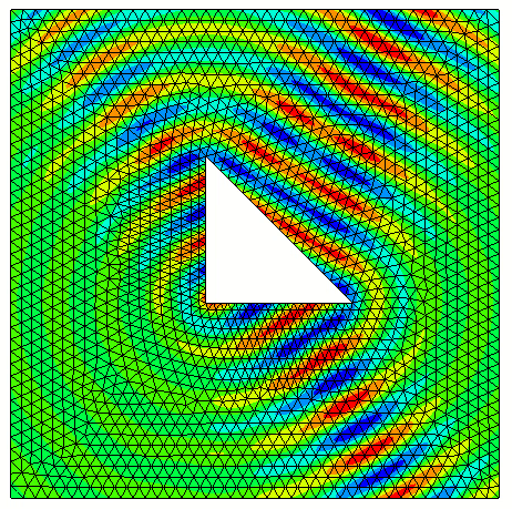
In this section we focus on the SSSP where $\Omega_{-}$ is a generic polygon, in particular choose as $\Omega_{-}$ a triangle which has barycenter in the origin. First we have to define the geometry of the problem using Netgen 2D Geometry library.

geo = SplineGeometry()
geo.AddRectangle((1,1),(-1,-1),bc="rectangle")
########################
#  TRIANGLE SCATTERER  #
########################
# In the following lines we define the triangle scatterer
gamma = 0.6; #Scaling factor of the (0,0)-(0,1)-(1,0) triangle.
def l(x):
    return -x+1;
M = 10; #Number of segments in which we split each side of the triangle.

#Adding the points to the mesh
pnts=[];
for i in range(0,M):
    pnts.append((0,i/M));
for i in range(0,M):
    pnts.append((i/M,l(i/M)))
for i in range(0,M):
    pnts.append(((M-i)/M,0));
#Shifting the points such that (0,0) is the barycenter 
TPnts = [(gamma*(p[0]-(1/3)),gamma*(p[1]-(1/3)))for p in pnts]
P = [geo.AppendPoint(*pnt) for pnt in TPnts]  
plt.scatter([p[0] for p in TPnts],[p[1] for p in TPnts])
#Connecting the points using streight segments.
Curves = [[["line",P[i],P[i+1]],"l"+str(int(i))] for i in range(0,len(pnts)-1)]
Curves.append([["line",P[len(pnts)-1],P[0]],"l"+str(int(len(pnts)-1))])

#Adding the midpoints of the segments to the mesh.
pnts2=[];
for j in range(0,3*M):
    if j in range(0,M):
        pnts2.append((pnts[j][0],pnts[j][1]+(0.5/M)));
    elif j in range(2*M,3*M):
        pnts2.append((pnts[j][0]-(0.5/M),pnts[j][1]));
    else:
        pnts2.append((pnts[j][0]+(0.5/M),pnts[j][1]-(0.5/M)))

#Shifting the points such that (0,0) is the barycenter 
TPnts2 = [(gamma*(p[0]-(1/3)),gamma*(p[1]-(1/3)))for p in pnts2]
P2 = [geo.AppendPoint(*pnt) for pnt in TPnts2]  
plt.scatter([p[0] for p in TPnts2],[p[1] for p in TPnts2],c="r")
plt.scatter(0,0,c="y")
#Connecting the points using streight segments.
Curves = []
for i in range(0,len(pnts)-1):
    Curves.append([["line",P[i],P2[i]],"m"+str(2*int(i+1)-1)])
    Curves.append([["line",P2[i],P[i+1]],"m"+str(2*int(i+1))])
Curves.append([["line",P[len(pnts)-1],P2[len(pnts)-1]],"m"+str(2*(len(pnts2))-1)])
Curves.append([["line",P2[len(pnts)-1],P[0]],"m"+str(2*(len(pnts2)))])

[geo.Append(c,bc=bc) for c,bc in Curves]

#Plot the mesh points and priting some measures.
plt.scatter(TPnts[0][0],TPnts[0][1],c="g")
plt.scatter(TPnts[M][0],TPnts[M][1],c="g")
plt.scatter(TPnts[2*M][0],TPnts[2*M][1],c="g")
print(TPnts[0][0],TPnts[0][1])
print((TPnts[2*M][1]-TPnts[M][1])/(TPnts[2*M][0]-TPnts[M][0]))
print(sqrt((TPnts[M+1][0]-TPnts[M][0])**2+(TPnts[M+1][1]-TPnts[M][1])**2),(gamma/M)*sqrt(2))
print(sqrt((TPnts[1][0]-TPnts[0][0])**2+(TPnts[1][1]-TPnts[0][1])**2),(gamma/M))
mesh = Mesh(geo.GenerateMesh(maxh=0.5/M)) #Meshing ...

plt.scatter(TPnts2[2*M-1][0],TPnts2[2*M-1][1],c="y")
#Defining polar coordinates
rho = sqrt(x**2+y**2);
theta = atan2(y,x)
Draw(theta,mesh,'theta')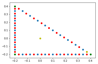

To do this we introduce the Helmholtz fundamental solution:

$\Phi_k(\vec{x},\vec{y}) = \frac{i}{4} H_0^1(k|\vec{x}-\vec{y}|),\qquad\qquad \forall \vec{x},\vec{y} \in \mathbb{R}^2 \; such\; that\;\vec{x}\ne \vec{y} .$

Any linear combination of the form $\sum_{j} \psi_j \Phi_k(\cdot,\vec{y_j})$ , where $\vec{y_j}\in\overline{\Omega_{-}}$ , is a radiating Helmholtz solution in $\Omega_{+}$ . We can take a continuous linear combination, focused on $\vec{y_j}\in \partial \Omega_{-}$ , to obtain a radiating Helmholtz solution:

$\label{eq:BIO}\mathcal{S}\psi (\vec{x}) = \int_{\partial\Omega_{-}} \psi(\vec{y})\Phi_k(\vec{x},\vec{y})ds(\vec{y})\qquad\qquad \vec{x}\in \Omega_{+}$

the operator $\mathcal{S}$ is called Helmholtz single layer potential.
We similarly define the single layer operator as follow:

$\label{eq:BIE}S\psi (\vec{x}) = \int_{\partial\Omega_{-}} \psi(\vec{y})\Phi_k(\vec{x},\vec{y})ds(\vec{y})\qquad\qquad \vec{x}\in \partial\Omega_{-}$

to find the potential $\psi$ that satisfy the previous equation we use a collocation method. In a collocation method we fix a discrete space $V_h\subset H^{-\frac{1}{2}}(\partial\Omega_{-})$ , in particular since $L^2(\partial\Omega_{-})$ is contained in $H^{-\frac{1}{2}}(\partial\Omega_{-})$ we like for $V_h$ to accommodate discontinuous functions. To build $V_h$ we divide $\partial\Omega_{-}$ in a number of elements $K_j$ , then we define $V_h$ as:

$V_h = <\varphi_1,\cdots, \varphi_{NDoF}>,\qquad\qquad \varphi_j(s) = \begin{cases}1\Leftrightarrow s \in K_j\0\Leftrightarrow s \in \bigcup_{i\ne j}K_i\end{cases}$

we can rewrite the second integral equation assuming that $\psi$ lives in $V_h$ , i.e. $\psi = \sum_{j}\vec{\psi}j\varphi_j$ :

$\sum{j} \vec{\psi}j \int{\partial\Omega_{-}}\Phi_k(\vec{x},\vec{y})\varphi_j(\vec{y}) ds(\vec{y})=g(\vec{x})$

we impose the previous equation on the midpoints of the segments $K_j$ to obtain the following linear system:

$A\vec{x} = \vec{b}\A_{ij} = \int_{\partial\Omega_{-}}\Phi_k(\vec{m_i},\vec{y})\varphi_j(\vec{y}) ds(\vec{y})=\int_{K_j}\Phi_k(\vec{m_i},\vec{y})ds(\vec{y})\b_i = g(\vec{m}_i)$

where $\vec{m}_i$ is the midpoint of the segment $K_i$ . Solving the linear system we obtain the vector $\vec{\psi}$ , and we can use first integral equation to compute the scattered wave:

$u_{st}(\vec{x}) = S\psi (\vec{x}) = \int_{\partial\Omega_{-}} \psi(\vec{y})\Phi_k(\vec{x},\vec{y})ds(\vec{y})=\int_{\partial\Omega_{-}}\sum_j\psi_j\varphi_j(\vec{y})\Phi_k(\vec{x},\vec{y})ds(\vec{y})=\\sum_{j}\psi_j\int_{K_j}\Phi_k(\vec{x},\vec{y})ds(\vec{y})$

#We here define a planar wave in the direction d=(0.5sqrt(3),0.5) with k=10.
# u(x) = exp(i(x°d)) = exp(ik*rho*|d|*cos(theta-pi/6))
k=30
def PW(Angle):
    pw = exp(1j*k*sqrt(x**2+y**2)*sqrt((0.5*sqrt(3))**2+0.25)*cos(theta-Angle));
    return pw;

N = 3*M; #Full number of segments
A = np.zeros((N,N),complex) #Init of the stifness matrix
F = np.zeros((N,1),complex) #Init of vector b, Ax=b.

for j in range(0,N):
    for i in range(0,N):
        #Computing Single Layer Potential with as one variable the mid points.
        HelmholtzSLP = CoefficientFunction(0.25*1j*sp.hankel1(z=k*sqrt((TPnts2[j][0]-x)**2+(TPnts2[j][1]-y)**2),v=0))
        #Integrating SLP to create the stifness matrix.
        A[i,j]= Integrate(HelmholtzSLP,mesh,definedon=mesh.Boundaries("m"+str(2*(i+1)-1)),order=20)+Integrate(HelmholtzSLP,mesh,definedon=mesh.Boundaries("m"+str(2*(i+1))),order=20); 
        if i in range(M,2*M):
            A[i,j] = (1/sqrt(2))*A[i,j]; #Correction factor due to NGSOLVE integration.
    mip = mesh(TPnts2[j][0],TPnts2[j][1]); #Defining mid point as mesh element
    #j-th components of b is the value of the planaer wave in the mid point
    F[j] = PW(pi/3)(mip);
print("Matrix Conditioning: ", np.linalg.cond(A))
Psi = np.linalg.solve(A,F) #Computing x

gamma=0.6 #Scaling factor of the (0,0)-(0,1)-(1,0) triangle.

def SLO(Psi):
    #We integrate using a mid point quadrature rule to obtain a function in one variable.
    u = 0*x+0*y; #Init u
    N=len(Psi);
    M =int(len(Psi)/3);
    for j in range(0,N):
        #We divide the integration among the three edge of the triangle
        if j in range(0,M):
            h = (gamma)*(1/M);
            plt.scatter(TPnts2[j][0],TPnts2[j][1],c="y")
            HelmholtzSLP = CoefficientFunction(0.25*1j*sp.hankel1(z=k*sqrt((TPnts2[j][0]-x)**2+(TPnts2[j][1]-y)**2),v=0))
        elif j in range(2*M,N):
            plt.scatter(TPnts2[j][0],TPnts2[j][1],c="g")
            h = (gamma)*(1/M);
            HelmholtzSLP = CoefficientFunction(0.25*1j*sp.hankel1(z=k*sqrt((TPnts2[j][0]-x)**2+(TPnts2[j][1]-y)**2),v=0))
        elif j in range(M,2*M):
            plt.scatter(TPnts2[j][0],TPnts2[j][1],c="r")
            dt = 1#sqrt(2) #On the hypotenuse we have a factor sqrt(2) to correct.
            h = (gamma/M)*dt
            HelmholtzSLP = CoefficientFunction(0.25*1j*sp.hankel1(z=k*sqrt((TPnts2[j][0]-x)**2+(TPnts2[j][1]-y)**2),v=0))
        u -=h*Psi[j][0]*HelmholtzSLP;
    return u;

Ust = SLO(Psi)
Uin = PW(pi/3)
Utot = Ust+Uin;
Draw(Uin,mesh,'Uin')

Draw(Ust,mesh,'Ust')
Draw(Utot,mesh,'Utot')

triag = SplineGeometry()
Del = (gamma)*(2/M);
triagpnts =[(-0.2+Del,-0.2+Del),(-0.2+Del,0.4-Del),(0.4-Del,-0.2+Del)]
p1,p2,p3= [triag.AppendPoint(*pnt) for pnt in triagpnts]
triag.Append(['line', p1, p3], bc='bottom', leftdomain=1, rightdomain=0)
triag.Append(['line', p3, p2], bc='right', leftdomain=1, rightdomain=0)
triag.Append(['line', p2,p1], bc='left', leftdomain=1, rightdomain=0)
TriagMesh = Mesh(triag.GenerateMesh(maxh=0.02,quad=True))

MIP = TriagMesh(-0.2+Del,-0.2+Del);
Ust = SLO(Psi)
Uin = PW(pi/3)
u = Ust+Uin;
Draw(u,TriagMesh,'u')
print(u(MIP))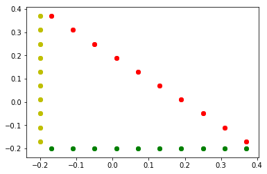

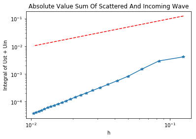
We now study the evolution of the quantity $|u_{St}+u_{In}|$ in the inside of the scatter knowing that inside of the scatterer $u_{St}+u_{In}$ is null.

err = [] #Init. vector of abs(Ust+Uin)
errI = [] #Init. vector of Integral Ust+Uin
H = [] #Init. of the diameter vector
IT = list(range(4,50,2));
#Computing Ust and Uin for each M.
for M in IT:
    geo = SplineGeometry()
    geo.AddRectangle((1,1),(-1,-1),bc="rectangle")
    gamma = 0.6;
    def l(x):
        return -x+1;

    pnts=[];
    for i in range(0,M):
        pnts.append((0,i/M));
    for i in range(0,M):
        pnts.append((i/M,l(i/M)))
    for i in range(0,M):
        pnts.append(((M-i)/M,0));
    TPnts = [(gamma*(p[0]-(1/3)),gamma*(p[1]-(1/3)))for p in pnts]
    P = [geo.AppendPoint(*pnt) for pnt in TPnts]  

    Curves = [[["line",P[i],P[i+1]],"l"+str(int(i))] for i in range(0,len(pnts)-1)]
    Curves.append([["line",P[len(pnts)-1],P[0]],"l"+str(int(len(pnts)-1))])


    pnts2=[];
    for j in range(0,3*M):
        if j in range(0,M):
            pnts2.append((pnts[j][0],pnts[j][1]+(0.5/M)));
        elif j in range(2*M,3*M):
            pnts2.append((pnts[j][0]-(0.5/M),pnts[j][1]));
        else:
            pnts2.append((pnts[j][0]+(0.5/M),pnts[j][1]-(0.5/M)))

    TPnts2 = [(gamma*(p[0]-(1/3)),gamma*(p[1]-(1/3)))for p in pnts2]

    P2 = [geo.AppendPoint(*pnt) for pnt in TPnts2]  


    Curves = []
    for i in range(0,len(pnts)-1):
        Curves.append([["line",P[i],P2[i]],"m"+str(2*int(i+1)-1)])
        Curves.append([["line",P2[i],P[i+1]],"m"+str(2*int(i+1))])
    Curves.append([["line",P[len(pnts)-1],P2[len(pnts)-1]],"m"+str(2*(len(pnts2))-1)])
    Curves.append([["line",P2[len(pnts)-1],P[0]],"m"+str(2*(len(pnts2)))])

    [geo.Append(c,bc=bc) for c,bc in Curves]


    mesh = Mesh(geo.GenerateMesh(maxh=0.5/M))

    rho = sqrt(x**2+y**2);
    theta = atan2(y,x)
    
    N = 3*M;
    A = np.zeros((N,N),complex)
    F = np.zeros((N,1),complex)

    for j in range(0,N):
        for i in range(0,N):
            HelmholtzSLP = CoefficientFunction(0.25*1j*sp.hankel1(z=k*sqrt((TPnts2[j][0]-x)**2+(TPnts2[j][1]-y)**2),v=0))
            A[i,j]= Integrate(HelmholtzSLP,mesh,definedon=mesh.Boundaries("m"+str(2*(i+1)-1)),order=10)+Integrate(HelmholtzSLP,mesh,definedon=mesh.Boundaries("m"+str(2*(i+1))),order=10); 
            if i in range(M,2*M):
                A[i,j] = (1/sqrt(2))*A[i,j];#Correction factor due to NGSOLVE integration.
        mip = mesh(TPnts2[j][0],TPnts2[j][1]);
        F[j] = PW(pi/3)(mip);
    print("Matrix Conditioning: ", np.linalg.cond(A))
    Psi = np.linalg.solve(A,F);
    
    
    triag = SplineGeometry()
    Del = (gamma)*(2/M);
    triagpnts =[(-0.2,-0.2),(-0.2,0.4),(0.4,-0.2)]
    p1,p2,p3= [triag.AppendPoint(*pnt) for pnt in triagpnts]
    triag.Append(['line', p1, p3], bc='bottom', leftdomain=1, rightdomain=0)
    triag.Append(['line', p3, p2], bc='right', leftdomain=1, rightdomain=0)
    triag.Append(['line', p2,p1], bc='left', leftdomain=1, rightdomain=0)
    TriagMesh = Mesh(triag.GenerateMesh(maxh=0.02))
    
    MIP = TriagMesh(-0.2+Del,-0.2+Del);
    Ust = SLO(Psi)
    Uin = PW(pi/3)
    u = Ust+Uin;
    print("IT: ",M," Raggio: ",0.5/M," Sum of Ust and Uin in (0,0): ",abs(u(MIP))," Integral: ",abs(Integrate(u,TriagMesh,order=10)))
    err.append(abs(u(MIP)))
    errI.append(abs(Integrate(u,TriagMesh,order=10)))
    H.append(0.5/M);

#Plot the graph of err vs H
plt.figure()
plt.plot(H,err,"*-")
plt.plot(H,H,"r--")

plt.title("Absolute Value Sum Of Scattered And Incoming Wave")
plt.ylabel("|Ust + Uin| in a point of the scatterer")
plt.xlabel("h")

plt.yscale("log")
plt.xscale("log")

print("Factor of convergence: ",log(err[-2]/err[-10])/log(H[-2]/H[-10]))

#Plot the graph of err vs H
plt.figure()
plt.plot(H,errI,"*-")
plt.plot(H,H,"r--")

plt.title("Absolute Value Sum Of Scattered And Incoming Wave")
plt.ylabel("Integral of Ust + Uin")
plt.xlabel("h")

plt.yscale("log")
plt.xscale("log")

print("Factor of convergence: ",log(errI[-1]/errI[-10])/log(H[-1]/H[-10]))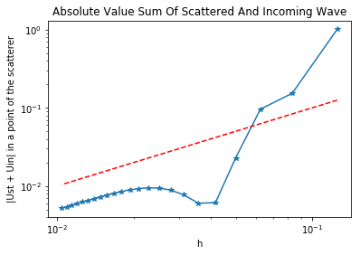

FEM and Truncated Problem

We now take a look at a different method aimed at solving the SSSP using finite element methods (FEM) rather then boundary element methods (BEM). The exterior Dirichlet problem is equivalent to the following PDE on a truncated domain $\Omega = B_R(\vec{0})\cap \Omega_{+}$ :

$\Delta u + k^2 u = 0\; in\; \Omega\gamma^{+}$

$u = g\; on\; \partial\Omega_{-}$

$DtN(\gamma^{+}u) -\partial_n u = 0 \; on \; \partial B_R(\vec{0})$

where the DtN is the operator defined as follow.

Definition

Given a function $g:\partial B_R(\vec{0})\to \mathbb{R}$ we can decompose $g$ in circular harmonics series, i.e Fourier series:

$g(\theta) = \sum_{l\in \mathbb{Z}} v_l e^{il\theta}$

the DtN operator acts as follow:

$DtN(g) = \sum_{l\in\mathbb{Z}} \frac{k H_l^{(1)}(kR)}{H_l^{(1)}(kR)} v_l e^{il\theta}$

this can be written in variational form as follow:

$Find\; u\in H^{1}{0}(\Omega) \; such \; that\; A(u,v) = F(v)\; \forall v \in H^{1}{0}(\Omega)$

$A(u,v) = \int_\Omega (\nabla u \overline{\nabla v} -k^2u\overline{v})\,d\vec{x} - \int_{\partial B_R} DtN(\gamma^{+}u)(\gamma^{+}v)\,ds$

$F(v) = \int_\Omega f\overline{v}\,d\vec{x}$

as $R$ grows to infinity we can replace the previous problem with the following:

$Find\; u\in H^{1}{0}(\Omega) \; such \; that\; A(u,v) = F(v)\; \forall v \in H^{1}{0}(\Omega)$

$A(u,v) = \int_\Omega (\nabla u \overline{\nabla v} -k^2u\overline{v})\,d\vec{x} - ik^2\int_{\partial B_R} u\overline{v},ds$

$F(v) = \int_\Omega f\overline{v}\,d\vec{x}$

Here we have imposed some conditions that mimics the radiating condition with an impedance condition that is equivalent to the radiating condition when $R$ grows to infinity.

geo = SplineGeometry()
geo.AddCircle((0, 0), 1,  bc="outer")
########################
#  TRIANGLE SCATTERER
########################
gamma = 0.6;
def l(x):
    return -x+1;

M = 10;
N = 3*M

pnts=[];
for i in range(0,M+1):
    pnts.append((0,i/M));
for i in range(1,M):
    pnts.append((i/M,l(i/M)))
for i in range(0,M):
    pnts.append(((M-i)/M,0));
TPnts = [(gamma*(p[0]-(1/3)),gamma*(p[1]-(1/3)))for p in pnts]
P = [geo.AppendPoint(*pnt) for pnt in TPnts]  

Curves = [[["line",P[i],P[i+1]],"l"+str(int(i))] for i in range(0,len(pnts)-1)]
Curves.append([["line",P[len(pnts)-1],P[0]],"l"+str(int(len(pnts)-1))])


pnts2=[];
for j in range(0,3*M):
    if j in range(0,M):
        pnts2.append((pnts[j][0],pnts[j][1]+(0.5/M)));
    elif j in range(2*M,3*M):
        pnts2.append((pnts[j][0]-(0.5/M),pnts[j][1]));
    else:
        pnts2.append((pnts[j][0]+(0.5/M),pnts[j][1]-(0.5/M)))
        
TPnts2 = [(gamma*(p[0]-(1/3)),gamma*(p[1]-(1/3)))for p in pnts2]

P2 = [geo.AppendPoint(*pnt) for pnt in TPnts2]  

Curves = []
for i in range(0,len(pnts)-1):
    Curves.append([["line",P[i],P2[i]],"m"+str(2*int(i+1)-1)])
    Curves.append([["line",P2[i],P[i+1]],"m"+str(2*int(i+1))])
Curves.append([["line",P[len(pnts)-1],P2[len(pnts)-1]],"m"+str(2*(len(pnts2))-1)])
Curves.append([["line",P2[len(pnts)-1],P[0]],"m"+str(2*(len(pnts2)))])

[geo.Append(c,bc=bc) for c,bc in Curves]


mesh = Mesh(geo.GenerateMesh(maxh=0.5/M)) #Meshing ...
#Defining polar coordinates.
rho = sqrt(x**2+y**2);
theta = atan2(y,x)

#We here define a planar wave in the direction d=(0.5sqrt(3),0.5) with k=10.
# u(x) = exp(i(x°d)) = exp(ik*rho*|d|*cos(theta-pi/6))
k=10
def PW(Angle):
    pw = exp(1j*k*sqrt(x**2+y**2)*sqrt((0.5*sqrt(3))**2+0.25)*cos(theta-Angle));
    return pw;
Uin = PW(pi/3)
Draw(Uin,mesh,'Uin'); #We plot Uin
#We define a H1 complex space with Dirichlet boundary condition on the circle edge.
fes = H1(mesh, order=1, complex=True,dirichlet="|".join(["m"+str(i) for i in range(1,2*N+1)]))
u, v = fes.TnT() #Trial and test functions

#We define the bilinear form.
a = BilinearForm(fes)
a += grad(u)*grad(v)*dx - k**2*u*v*dx
a += -k*1j*u*v * ds("outer") #Impedence condition
a.Assemble()

#Linear application
f = LinearForm(fes)
f += 0 * v * dx
f.Assemble()

uh = GridFunction(fes, name="uh") #Init. Ust
uBND = GridFunction(fes, name="UinBnd") #Init. Uin on the boundary
uh.Set(Uin,BND) #Setting Boundary condition
uBND.Set(Uin,BND) #Setting Boundary condition
Draw(uBND,mesh,"UinBND") #Plotting Uin on the boundary

#Solving fot Ust
r = f.vec.CreateVector()
r.data = f.vec - a.mat * uh.vec
uh.vec.data += a.mat.Inverse(freedofs=fes.FreeDofs()) * r
#Drawing Ust and Ust-Uin
Draw(uh,mesh,'uh')
Draw(uh-Uin,mesh,'utot')

UZ Blog

BEM For Helmholtz Sound-Soft Scattering Problem

Definition – Radiating Helmholtz Solution

Definition – Exterior Dirichlet Problem

Definition

Example – SSSP and Circular Scatterer

Triangular Scatterer and Collocation BEM

FEM and Truncated Problem

Definition

Related Posts

Turing Patterns

Dahlquist Barrier and Symplectic Integrator For Time-Stepping The Wave Equation

Conjugated Gradient an Optimal Stopping Time Approach

Leave a Reply Cancel reply