Introduction
Suppose that we have a symmetric matrix  and our aim is to solve the linear problem
  to find the exact solution
  . One of the algorithm widely implemented to perform such task is the conjugated gradient (CG) method. The standard formulation of the CG method is as follow:
- We define the initial step:
 .
. - We compute the length of our next step:
 .
. - We compute the approximated solution:
 .
. - We compute the residual:

- Last but not least we update the search direction:

the idea behind this method is to find the best the approximation  in the Krylov subspace of order
  ,
,  , that minimize the quantity:
  . A couple of interesting result for the CG method are the following:
Theorem 1
The following statements holds when the CG method is applied to a symmetric matrix:
 .
. - The residual are orthogonal:
 .
. - The search directions are
 conjugated:
Theorem 2
If we apply the CG method to a positive defined symmetric matrix the element  that minimize
  is unique and the converge with respect to:

is monotonic.
More detail on the CG method and the theorems before mentioned can be found in Numerical Linear Algebra, Lloyd N. Trefethen. An interesting aspect is that even if Theorem 2 states that the error of the CG in the norm induced by is monotonically decreasing, we can’t state the same for the residual  . In the next sections we will try to use techniques developed in the field of optimal stopping time to address the question of when is convenient to arrest our method in order to minimize the residual.
Preliminary Example
Let’s begin by addressing a very simple problem, suppose that we can compute steps of the CG and we have reached the step  . How can we decide if would be convenient in terms of residual to compute the -th step ? Well a straight forward answer would be that we should compute if:
![\mathbb{E}\Big[||A\vec{\xi_n} - \vec{b}||\Big]< ||\vec{r_{n-1}}||\;\;\;\; (D1)](https://www.uzerbinati.eu/wp-content/ql-cache/quicklatex.com-c9675d7fe3b106354d6626996de6bafa_l3.png "Rendered by QuickLaTeX.com")
where  is the random variable whose realization is and we can use any norm of our choosing, with out altering much the meaning of the equation. Considering the fact that each step of the CG method is computed only considering thee previous we can assume that is a Markov process. In light of the fact that is Markov chain we can replace as decision criteria
  with:
with:
![\mathbb{E}\Big[||A\vec{\xi_n} - \vec{b}||\; \Big| \; \vec{\xi_{n-1}}=\vec{x_{n-1}}\Big]< || \vec{r_{n-1}}||\;\;\;\; (D2)](https://www.uzerbinati.eu/wp-content/ql-cache/quicklatex.com-1ca1a38f06b45b7171e35829eb85ec09_l3.png "Rendered by QuickLaTeX.com")
The idea of introducing is justified by the fact that the value that of is unknown to the user at time even if it can be exactly computed at the -th step. The idea is for the user to make and “educated guess” of the out come for the CG method at step , and to decide thanks to this educated guess if proceed to compute . The “education” of our guess consist in the distribution that we assume has. We know that the CG method moves along a direction  of length
  to minimize
  and we need to find a distribution that correctly represent this behavior. To do so we start from a multivariate Gaussian in
  centered in
  :
:

Then we puncture the Gaussian propagating it using the wave equation:

the solution of the above problem that we will denote as  still is a probability density function under certain hypothesis that we will investigate later. Furthermore it has the shape of a punctured Gaussian. Such a shape tell us that we have greater probability of finding around the
  -dimensional hole produced around . In particular since we known that the wave front propagate as sphere of radios
  in the particular case of Gaussian pulses, the density
  seems a fear distribution for given that we have
  . We should remark latter on how spectral properties of together with the choice of
  can improve the way we build our distribution, we will remark in the same section that we can provide a general formula to compute
  . Now if we decide to use the euclidean norm to evaluate our residual we have that
  is equivalent to:


Equation  tell us when is convenient to compute according to our
 educated guess.
Further Discussion Regarding The Distribution
Here we wont to extend the explanation to why the distribution  was chosen together with some general remarks regarding it. We will start from a two dimensional view to ease our minds, or at least mine. We can image the CG method as moving from
  to
to  along the direction
  with length
  . So we can start assuming that
  is distributed around
  with radius . But clearly we wont the density function of to be null near
  since we know we are moving away from it. To achieve this result we began from a Gaussian centered in :

then we propagate this distribution using the wave equation. In particular we are interested in finding the solution to the problem:

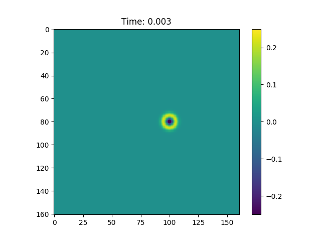
Figure 1, In figure is possible to observe how the wave equation propagates a Gaussian pulse. 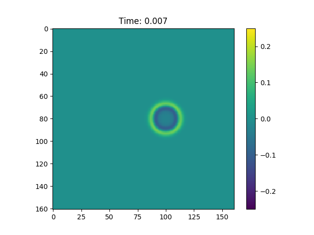
Figure 1, In figure is possible to observe how the wave equation propagates a Gaussian pulse. 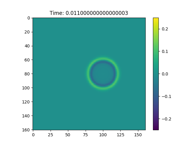
Figure 1, In figure is possible to observe how the wave equation propagates a Gaussian pulse.
We can see from Figure 1 that this procedure creates a hole in our normal distribution, and this hole expands with time. Furthermore if we consider the Green function associated with this problem:

where  is the Heaviside function. We can easily see that the radius of the ”hole“ produced propagating
  using the wave equation is
  since:

We can as well compute explicitly the solution to the wave equation:


we consider only the absolute value part of this function to obtain a function  that is Lebesgue integrable and non-negative, ie it is a probability density function if we normalize. In particular we will call
  the probability density function obtained this way. We can do the same procedure for a Gaussian of
  , and we can compute analiticaly the solution to the wave propagation, as in Wave Equation in Higher Dimensions, Lecture Notes Maths 220A Stanford, to see that we have a Lebsgue integrable. We will call
  the pdf obtained by the normalization of the absolute part of the previously mentioned solution with
  , starting from a Gaussian centered in . Furthermore even in higher dimension we know that the wave front propagates at a distance from the mean of the Gaussian, and so we will have an hole of radius , produced in the center of the Gaussian.
Last but not least since we know the direction of search we can choose such that it has eigenvector  and that this eigenvector is associated with the greatest eigenvalue of the matrix. This produced the Gaussian shown in Figure 2.
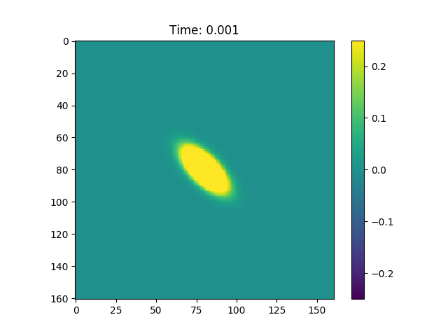
Figure 2, In figure is possible to observe a Gaussian that propagates in the direction of the CG search direction. 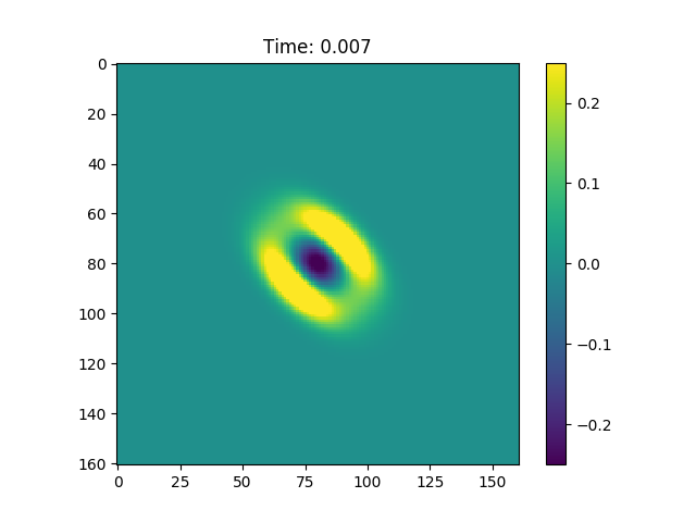
Figure 2, In figure is possible to observe a Gaussian that propagates in the direction of the CG search direction. 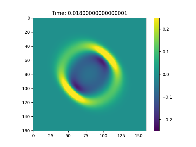
Figure 2, In figure is possible to observe a Gaussian that propagates in the direction of the CG search direction.
The last notation we will adopt is  to indicate the probability density function obtained using the direction of search as above, of radius but starting from a Gaussian centered in
  , propagated until .
Optimal Stopping Approach
We will here address the problem of finding the optimal stopping time for the CG method within a finite horizon  .
.
Let’s consider again the Markov chain  , we can suppose as we have done in our preliminary example that that
  . Here we have to deal with a time in-homogeneous therefore to apply the result developed in the book Optimal Stopping and Free-Boundary Problems, Peskir, Goran, Shiryaev, Albert N, we need to introduce a time homogeneous Markov chain:
  . Now to find the optimal stopping time for the CG method we will introduce a week version of the result presented in Optimal Stopping and Free-Boundary Problems, Peskir, Goran, Shiryaev, Albert N.
Theorem 3
Let’s consider the optimal stopping time problem:
![V^{m}(n,\vec{x}) = \underset{0\leq \tau \leq m-n}{\sup} \mathbb{E} \Big[ G(n+\tau,\xi{n+\tau}) \Big| \xi_{n} = \vec{x} \Big]](https://www.uzerbinati.eu/wp-content/ql-cache/quicklatex.com-756bf113558c54b179942ef00cad53d4_l3.png "Rendered by QuickLaTeX.com")
Assuming that ![\mathbb{E}\Big[ \underset{0\leq \tau \leq m-n}{\sup} |G(n+\tau,\xi_{n+\tau})| \Big] < \infty](https://www.uzerbinati.eu/wp-content/ql-cache/quicklatex.com-5c4db5eef5555be57ad5724a12b7e0c6_l3.png "Rendered by QuickLaTeX.com") , where
, where  is our gain function, then the following statements holds:
- The Wald-Bellaman equation can be used to compute:
![V^{m}(n,\vec{x}) = \max\bigg\{ G(n,\vec{x}), T\Big[ V^{m}(n,\vec{x}) \Big]\bigg\}](https://www.uzerbinati.eu/wp-content/ql-cache/quicklatex.com-87d751417e154b77e07d4612450914df_l3.png "Rendered by QuickLaTeX.com") for
for  .
. - The optimal stopping
 can be computed as:
  , where
  .
.
Then we can define the transition operator as follow:
![T\Big[ g(n,\vec{x}) \Big] = \mathbb{E} \Big[ g(n+1,\xi_{n+1}) \,\Big|\, \xi_n=\vec{x} \Big]](https://www.uzerbinati.eu/wp-content/ql-cache/quicklatex.com-9561575ca74318bdfa3b35d0a19affc9_l3.png "Rendered by QuickLaTeX.com")
In this case our gain function will be defined as follow:


which respect the hypothesis of the previous theorem since the greatest the gain function could get is  . Our transition operator becomes:
![T\Big[ g(n,\vec{x}) \Big] = \int_{\mathbb{R}^N} g(n+1,\vec{y})u_{n,\vec{x}}^{N}(\vec{y},\alpha_n) d\vec{y}](https://www.uzerbinati.eu/wp-content/ql-cache/quicklatex.com-8b4cbe32c8c403acdce5aab11b827699_l3.png "Rendered by QuickLaTeX.com")
In particular we can use Wald-Bellman equation to compute with a technique known as backward propagation  (this is a common practice in dynamical programming):


and this allows to build the set  , which inf is the optimal stopping time we were searching fore.
Conclusion
We have here shown two ideas, the first one is presented in section 2 and explain how to decide at step if is convenient to compute , the second one provide a technique to compute the optimal stopping time for the CG method. Those idea are just an interesting exercise on the optimal stopping time and a probabilistic approach to the arrest criteria for numerical linear algebra. This because to compute the density  and we need to have
  and that are the most complex operation in the CG method,
  .
.
An interesting approach to make the second idea computationally worth while would be the one of using a low-rank approximation of order  . In this way the complexity to compute the approximation of and is only
  .
.
Last but not least is important to mention that if we would like to implement the afore mentioned ideas we could use a Monte Carlo integration technique to evaluate the integrals in equation and  and a multi dimensional root-finding algorithm to find compute
  .
.
Interesting aspect that are worth investing are how to build the best possible low-rank approximation and if theory such as the one of generalized Toepliz sequences can give us useful information to build our density function in a more efficient way.